Sig2Lead aims to facilitate drug discovery and re-purposing by combining transcriptional signature connectivity analysis with cheminformatics approaches. In the first step, putative inhibitors of a target gene specified by the user are identified as those drug-like molecules in LINCS that have signatures concordant with a KD signature of the target. Note that LINCS arguably represents the largest resource for pharmacogenomics to date, with over 20,000 small molecules and about 5,000 gene KDs transcriptionally profiled, thus covering a large subset of the drug-like chemical space and druggable subset of the genome. In the second step, a set of additional candidate molecules, e.g., identified by virtual or experimental screening, can be ranked based on their chemical similarity to ‘concordant’ LINCS analogs using a fast chemical similarity search. Furthermore, Sig2Lead can be used to prepare input files for docking simulations to be performed in conjunction with connectivity-based analysis to improve the specificity of the search (see paper below), as well as identify LINCS analogs of user provided compounds irrespective of their connectivity to a target of interest. For a graphical overview of Sig2Lead see figure 1 below.

A diagram of a process

Description automatically generated

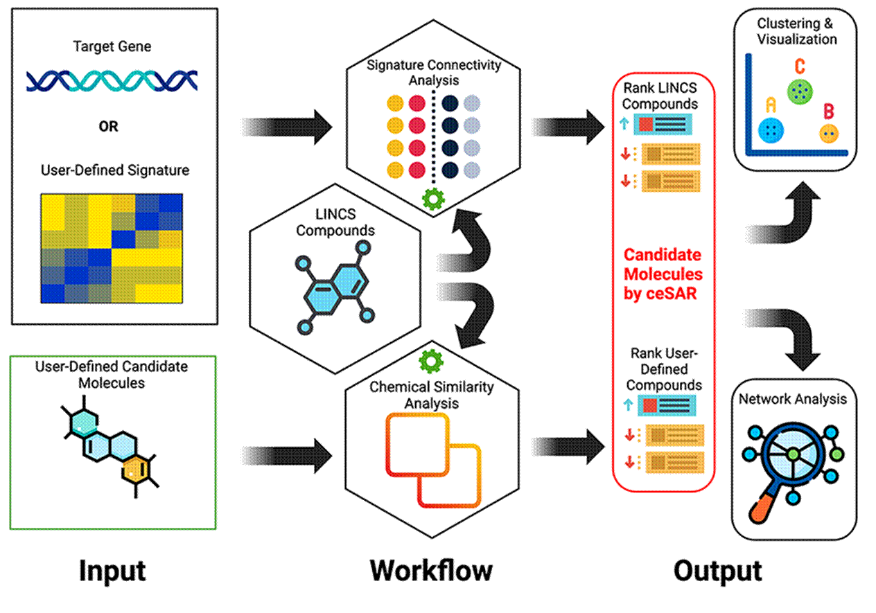
Figure 1: Sig2Lead Overview

Reference

Please cite the following paper that describes the signature connectivity and chemical similarity analyses for drug discovery implemented in Sig2Lead:

Thorman, A. W., Reigle, J., Chutipongtanate, S., Shamsaei, B., Pilarczyk, M., Faze l -Najafabadi, M., ... & Meller, J. (2020). Accelerating Drug Discovery and Repurposing by Combining Transcriptional Signatur e Connectivity with Docking . bioRxiv .

Paper Abstract

The development of targeted treatment options for precision medicine is hampered by a slow and costly process of drug screening. While small molecule docking simulations are often applied in conjunction with cheminformatic methods to reduce the number of candidate molecules to be tested experimentally, the current approaches suffer from high false positive rates and are computationally expensive. Here, we present a novel in silico approach for drug discovery and repurposing, dubbed connectivity enhanced Structure Activity Relationship (ceSAR) that improves on current methods by combining docking and virtual screening approaches with pharmacogenomics and transcriptional signature connectivity analysis. ceSAR builds on the landmark LINCS library of transcriptional signatures of over 20,000 drug-like molecules and ~5,000 gene knock-downs (KDs) to connect small molecules and their potential targets. For a set of candidate molecules and specific target gene, candidate molecules are first ranked by chemical similarity to their ‘concordant’ LINCS analogs that share signature similarity with a knock-down of the target gene. An efficient method for chemical similarity search, optimized for sparse binary fingerprints of chemical moieties, is used to enable fast searches for large libraries of small molecules. A small subset of candidate compounds identified in the first step is then re-scored by combining signature connectivity with docking simulations. On a set of 20 DUD-E benchmark targets with LINCS KDs, the consensus approach reduces significantly false positive rates, improving the median precision 3-fold over docking methods at the extreme library reduction. We conclude that signature connectivity and docking provide complementary signals, offering an avenue to improve the accuracy of virtual screening while reducing run times by multiple orders of magnitude.

Installation of Sig2Lead_v2.3

Introduction

Sig2Lead is available as a Shiny app to be executed in RStudio or as a docker container to be executed in a system-independent manner. The RStudio version is available on Github and the dockerized version is available on Docker Hub. The RStudio version requires that R and RStudio be locally installed on the user’s computer and requires the installation of all requisite R packages. The dockerized version requires installation of docker and Sig2Lead image. Once the Sig2Lead image is running, a web browser is used to run the app without the need to install R, RStudio, or all necessary R packages. This manual provides step-by-step instructions for both versions.

Installation/Configuration of RStudio Version

A. Install R and RStudio

Sig2Lead was built with R version 4.4.0 and is expected to run with any later versions of R (to avoid R dependencies please see dockerized version). The latest version of R can be downloaded at:

http://www.r -project.org /

Additionally, RStudio is required and can be downloaded at: https://www.rstudio.com/products/rstudio/download /

B. Download Sig2Lead from Github

Sig2Lead and associated files can be downloaded from:

https://github.com/sig2lead/sig2lead_v2.3/

Navigate to the Sig2Lead_v2.3 repository, click on “Code”, and select “Download Zip”. The downloaded zip file needs to be unzipped to a user-selected directory.

C. Install Required Libraries

Once R and RStudio are installed, shiny must be installed. This can be completed by typing into the R console:

install.packages(“shiny”)

All other dependencies and libraries will be installed upon the first time running the application.

This step may not be handled properly on MacOS, requiring a step-by-step installation of missing libraries. An alternative for Mac users is to use the dockerized version that takes care of all the dependencies.

To run the application, click the button at the top middle of the RStudio interface.

Installation of Dockerized Version

A. Install Docker

Ubuntu: follow the instruction s to get Docker CE for Ubuntu.

Mac: follow the instruction s to install the Stable version of Docker C E on Mac. Windows: follow the instruction s to install Docker Toolbo x on Windows.

For list of useful docker commands please see:

https://www.digitalocean.com/community/tutorials/ho w -t o -remov e -docke r -image scontainer s an d -volume s

B. Open Command Prompt

Open a command prompt using Powershell for Windows machines or a terminal window for Macs. On

Windows machine, click on the Start Menu, click on the “Windows Powershell” folder and tap “Windows PowerShell”. An alternative method is to go to the search bar in the lower left corner of the screen and input “Powershell”, which will display a menu option to choose and open “Windows Powershell”. On

Mac, launch Spotlight Search by clicking on the magnifying glass icon in the menu bar (or press Command+Space). When the Spotlight Search bar pops up on your screen, type “terminal.app” and hit Return. This will open a terminal.

C. Download Sig2Lead Container from Docker Hub

To download the docker image run the following command in a command prompt:

docker pull sig2lead/sig2lead:v2_3

Linux users may need to use sudo to run Docker by typing: sudo docker pull sig2lead/sig2lead:v2_3

Note that the Sig2Lead image is available from Docker Hub at http://hub.docker.com/repositories/Sig2Lead /

D. Run Sig2Lead Container

To run Sig2Lead container, open a command prompt and run following command:

docker run -p 3838:3838 -d sig2lead/sig2lead:v2_3

Before running the container make sure that port 3838 is free to run. You can stop and kill any other docker containers on this port by

[sudo] docker stop <container ID> && docker rm <container ID>

To check the container ID run this command:

docker ps -a

E. Open browser and navigate to localhost:3838

Open browser and navigate to the following url: http://127.0.0.1:3838

F. Run app following instructions below

Follow the instructions below for running the app.

Connectivity Analysis Tab

In the next several sections, several distinct workflows organized in 3 different tabs are discussed and illustrated using use cases. The first of those sections below describes the main tab where the primary workflow can be initiated by defining the target gene.

A. Define Target Gene Workflow

This is the standard workflow for identifying small molecule inhibitors or activators of a target of interest. Within this workflow, a gene of interest is required and optionally, a user-defined list of candidate compounds for scoring can be provided in SDF or SMILES format. Sig2Lead collects data from genetic knockdowns within LINCS and identifies compounds that generate highly concordant transcriptional signatures to these genetic knockdowns, i.e., putative target/pathway inhibitors. That step is dependent on ilincs.org API calls and requires Internet connection.

If an external set of candidate molecules is provided, e.g., identified by virtual or experimental screening, these user-provided candidate molecules are ranked based on their chemical similarity to ‘concordant’ LINCS analogs using a fast chemical similarity search. This method allows scoring of small molecules to be tested for the purpose of library reduction. Results for user added compounds will be ranked in descending order of similarity to ‘concordant’ LINCS analogs, with ties broken by concordance scores in the table titled “My Candidates Ranked”. Candidate compounds identified from within the LINCS library as concordant to a target KD will be scored only by their concordance scores (obtained from ilincs.org) to a knockdown of the target gene of interest in the table titled “LINCS Compounds Ranked”. These tables can be downloaded using the download buttons just below the “Go!” button. See Figures 2 and 3 below.

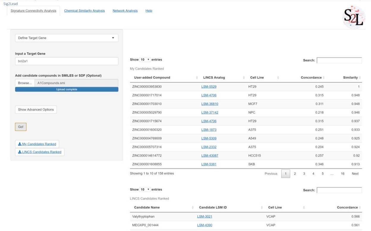
Figure 2: Define Target Gene workflow. In this primary workflow, the user defines a gene of interest to identify putative pathway/target inhibitors. If the user defines a set of compounds from some other analyses, those compounds will be compared to the LINCS library for analogous compounds and scored by similarity and concordance in the upper table (My Candidates Ranked), which will only appear in the event of added compounds. The lower table (LINCS Candidates Ranked) will always appear when running this workflow and scores all LINCS compounds with a concordance above the threshold in descending order of concordance.

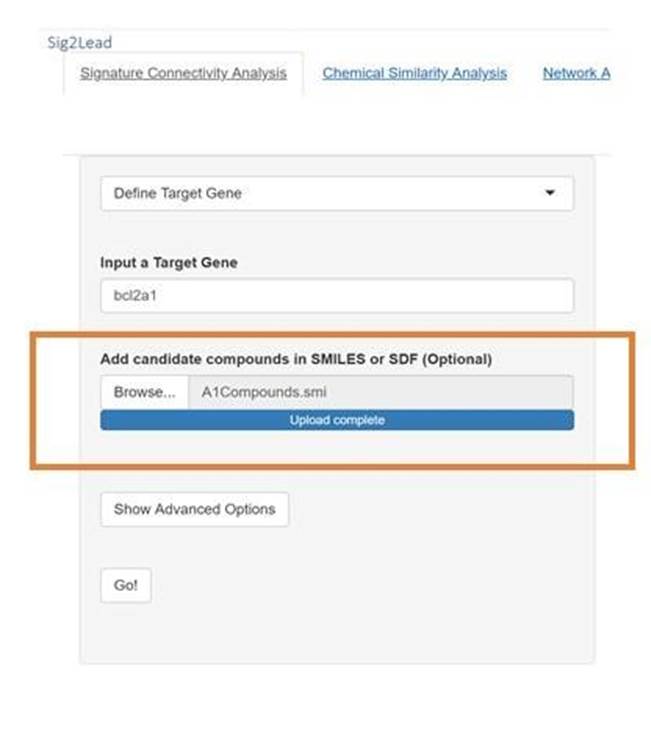
Figure 3: The file input for the RStudio version is shown in the above figure. The control has a standard upload control in which the user can press the “Browse” button and navigate to the directory with the “.smi” or “.sdf “files of userprovided compounds.

B. Upload a Signature Workflow

This workflow allows users to upload a signature of their own to search for potential inhibitors to a target gene unavailable on LINCS, or molecules that generate a similar signature to some other system perturbation that is otherwise undefined. In this workflow, users define a signature using one of the formats defined at (www.ilincs.org/ilincs/signatures/main /). This pipeline otherwise follows the same pipeline as the “Define Target Gene” workflow.

Graphical user interface, table

Description automatically generated

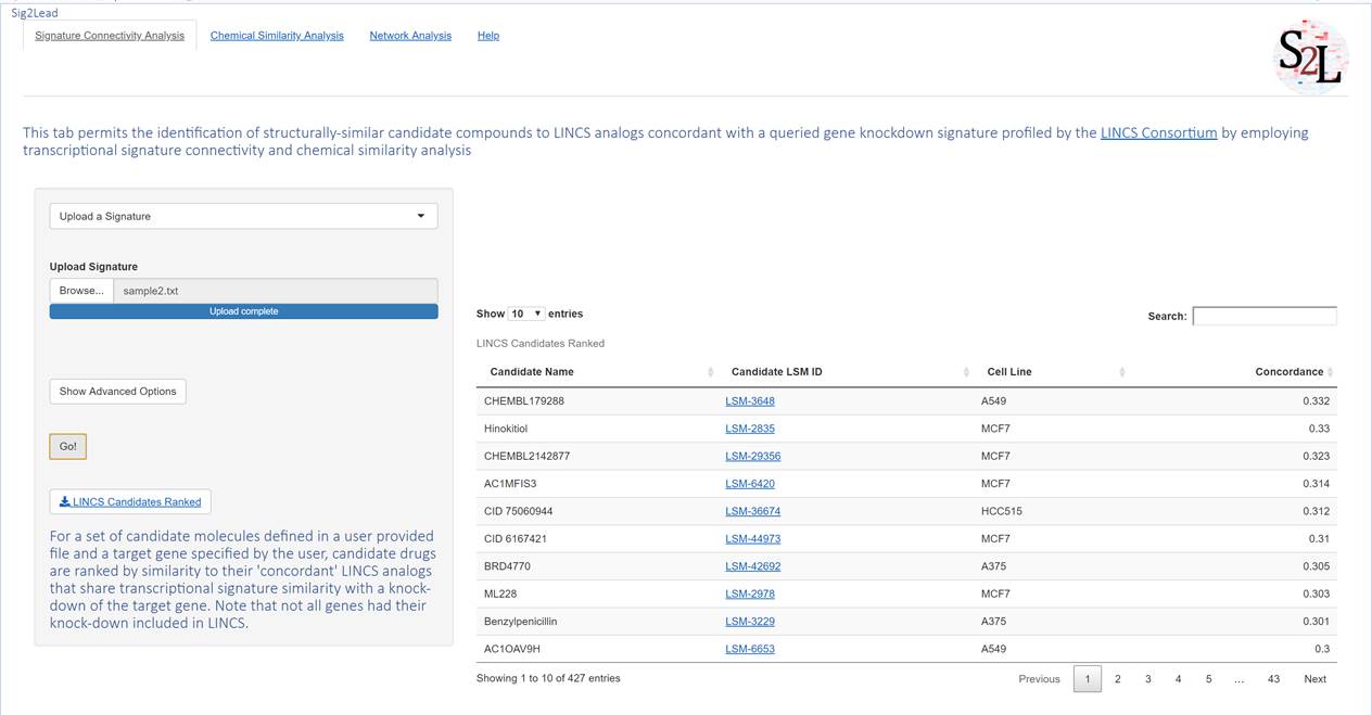
Figure 4. Upload a Signature Workflow. This workflow allows one to query iLINCS (see ilincs.org) to find small molecules in LINCS that have signatures concordant with a user provided transcriptional signature. The signature file should be saved as a tab-separated text file with gene symbol, log of differential expression value, and p-value comprising the columns in the that order. The output of this workflow is a table of ‘concordant’ LINCS small molecules that have transcriptional signatures similar to the uploaded signature.

C. Find Analogs in LINCS Workflow

This workflow simply identifies LINCS analogs to user-defined compounds, irrespective of their connectivity to a target. This requires added compounds and is useful in determining if there are transcriptionally profiled analogs in the LINCS library. LINCS compounds are drug or drug-like, many of them with known Mode of Action (MOA), so this may also be used as a simple filter to remove compounds that do not contain normal drug-like structures. Additionally, it was used in benchmarking as a baseline similarity of various compound libraries to the LINCS small molecules (see the reference paper).

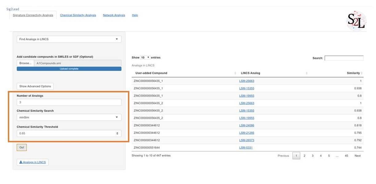
Figure 5: Find Analogs in LINCS Workflow. This workflow allows the user to find small molecules included in LINCS library that are structurally similar to user-provided compounds. The Advanced Options can be used to change the number of LINCS analogs to be returned for each user-provided compound, bounded by the chemical similarity threshold (also adjustable). The user can also use either the ultrafast minSim algorithm or slower fpSim algorithm to compute chemical similarity.

D. Advanced Options

A. Users can select options to identify either inhibitors or activators. Functionally, selecting activators results in searching for molecules that are discordant to the gene knockdown of interest instead of concordant.

B. Users can change the method used for similarity search. The default, minSim is an exact fast chemical similarity search utilized by Sig2Lead introduced in the reference paper. For comparison, an established fpSim function to compute chemical similarity is available as a slow option (it typically runs about 100x slower than minSim).

C. Finally, users can select the version of the iLINCS database to query. The choices are “Current” which is the latest version of iLINCS or the “Legacy” version which is the previous version. The concordance threshold can be changed also. The default is 0.1. For “Current“ iLINCS, the minimum concordance value observed is 0.162, while for “Legacy” iLINCS the minimum concordance threshold observed is 0.2. For some targets, a more stringent cutoff may be required to increase the specificity.

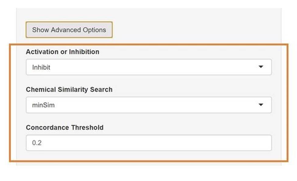
Figure 6. Define Target Gene Workflow Advanced Options.

E. User-Provided Candidate Compounds

A user-provided set of candidate compounds can be provided in either sdf or smiles format. Smiles files should be tab-delimited text files with the smiles in the first column and the labels in the second column. Acceptable file extensions for the smiles file include .smi and .txt.

Chemical Similarity Analysis Tab

After searching LINCS for ‘concordant’ analogs of user provided candidate compounds, both LINCS and user provided compounds can be further analyzed through chemical similarity using the “Chemical Similarity Analysis” tab. To run chemical similarity analysis click the “Run SAR” button. This will initiate a clustering analysis that compares concordant compounds from LINCS for the target and user-added compounds and clusters them by chemical similarity to one another. By default, 5,000 compounds will be analyzed (this can be changed under advanced options if an extended time is acceptable). The output will be in the form of two figures, a heatmap and an MDS plot, and a table of centroids for each cluster. The heatmap is generated through hierarchical clustering and shows a distance matrix comparing each compound identified through LINCS (Green) or added by the user (Blue). The MDS plot is an alternative view and implicit clustering by projection into 2D, showing relative distances between clusters of compounds. The radius of each pie chart corresponds to the size of the cluster.

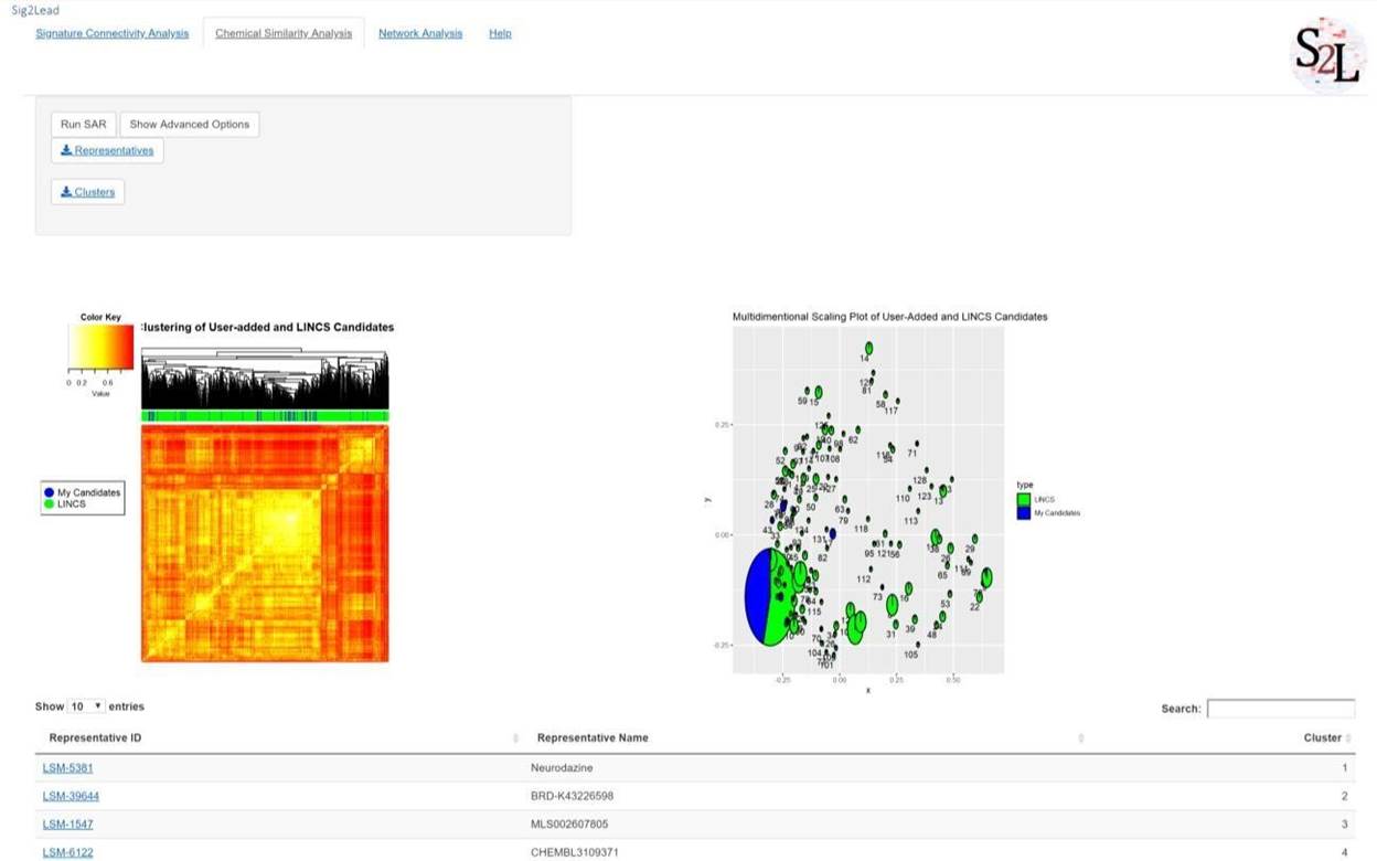
Figure 7. Example of chemical similarity analysis. SAR type analyses can be performed for either

‘concordant’ LINCS compounds (here shown in Green), or user provided candidate molecules (here in Blue), or together to identify distinct classes of chemical moieties within the set of user-provided compounds and their ‘concordant’ LINCS analogs. The heatmap in the left panel shows pairwise chemical similarity pattern with the compounds analyzed as both columns and rows, i.e., the diagonal represents identity (Tanimoto coefficient of 1.0). Note that user defined candidates indicated by blue ticks in the top bar are scattered throughout, i.e., they belong to several distinct classes of compounds with most of them in the middle ‘big’ cluster indicated by a large rectangular block of high similarity scores in the middle of the heatmap. This is further highlighted in the right panel that shows individual clusters identified using the MDS 2-dimensional projection of pairwise similarities, with the ‘big’ circle in the bottom left corner corresponding to the central mixed cluster in the heatmap.

A. Chemical Similarity Analysis Options

A. For clustering, different Tanimoto similarity thresholds can be selected. The default is 0.75, which groups compounds of modest difference together, but can be adjusted to make more (closer to 1) or less stringent clusters (closer to 0). This will only be reflected in the MDS plot and the table of representatives.

B. The minimum cluster size for inclusion in the MDS plot can also be changed. The user can cluster all compounds regardless of cluster size or increase this threshold to only consider those from large clusters of related compounds.

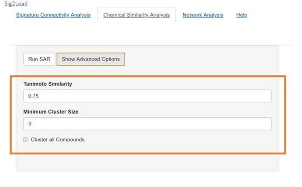
Figure 8. Chemical Similarity Analysis Advanced Options

Network Analysis Tab

Finally, Network connectivity analyses can be performed after chemical similarity analyses using STITCH on the “Network Analysis” tab. This analysis is intended to scrape any known information about identified compounds and their interactions with members of the pathway of interest. This step can be performed either through a global view (all identified compounds) or on a cluster-by-cluster basis (much faster).

For cluster-by-cluster analysis, select “Cluster Network STITCH” from the drop-down box. Following this click the “View Selected Cluster Network” button to see the gene-chemical interaction network of the specific cluster number (by default, the cluster number is set to 1) of the MDS plot from the “Chemical Similarity Analysis” tab (Figure 9).

When selecting “Global STITCH” from the drop-down box, all compounds found in clusters of sufficient size, as determined from the “Chemical Similarity Analysis” tab’s advanced options, will be included in the network analysis. If the “Shows all clusters” box is checked, all compounds are included regardless of the size of the cluster of which they are in. The Global STITCH analysis can be slow, depending on the number of compounds added.

This network analysis can help the user map the added compounds or the LINCS analogs of the selected cluster as target or pathway inhibitors. As an example, target inhibitors that directly interact with BCL2A1 as the target gene are shown in Figure 8. The molecules included are the user-added compounds and their LINCS chemical analogs based on the MDS clustering for the selected cluster.

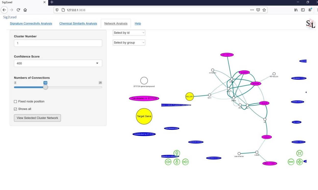
Figure 9: STITCH network analysis for BCL2A1 (the target gene showed as a yellow node) and associated chemicals, with the user-added compounds and their ‘concordant’ LINCS similar analogs showed as the magenta nodes. The edge between nodes represents their corresponding interactions based on the experimental evidence and text mining retrieved from the STITCH database.

Example Use Case

This use case demonstrates the screening for putative inhibitors of EGFR with a set of user provided candidate compounds.

1. In the “Input a Target Gene” box, type EGFR

2. For "Added candidate compounds", this demo will use the known EGFR active ligands downloaded from the DUD-E database

(http://dude.docking.org/targets/egfr/actives_final.sdf.g z ). Please browse to upload “EGFR_actives_final.sdf” which is already provided in the Sig2Lead folder.

3. Click the advance options button. The users will see three options show up here. Please choose “Legacy”, "Inhibit", "minSim”, and “0.3” for these options (as shown in Figure 9), and then click Go!

4. Once the analysis is finished, two tables will show up. The first table contains the similarity scores between the added compounds and their ‘concordant’ LINCS analog (the last column). The similarity of 1 for a user provided compound indicates that it was in fact included in the LINCS library and directly profiled. The second table shows ranking of LINCS candidates as potential EGFR targeted/pathway inhibitors based on their concordance score.

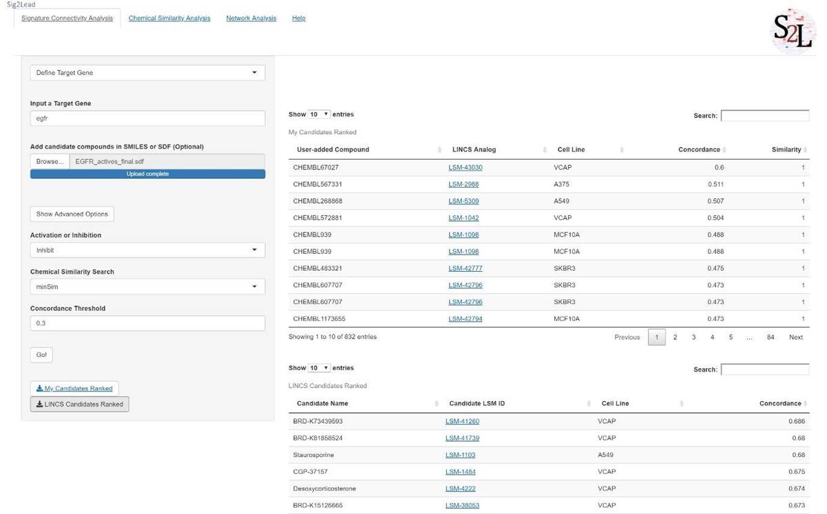
Figure 10. Signature Connectivity Analysis using EGFR as the target gene.

5. Next, go to the “Chemical Similarity” tab and click “Run SAR” button. This step may take a while.

6. Once finished, a heatmap and a multidimensional scaling plot will be generated (Figure 11). Both plots represent the added compounds in blue and LINCS compounds in green. These compounds are present in the same cluster based on their chemical similarity. To change the chemical similarity threshold for this analysis, please click "Show Advanced Options" button.

7. A table below the plots contains the representatives (centroids) of each MDS cluster. To download the full table result, please click “Representatives” button. Here, the users can retrieve LINCS compounds that may share the same activity as the user-added candidate compounds.

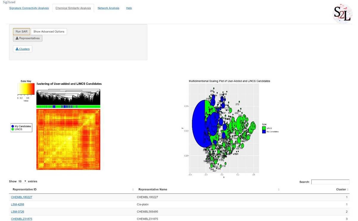
Figure 11. Chemical similarity analysis of user-added compounds against LINCS chemicals. Blue and green colors are used to label the user-added compounds and LINCS analogs, respectively, in the heatmap (left) and the MDS plot (right).

8. Finally, go to the “Network Analysis” tab to perform gene-chemical interaction network analysis based on known interactions (from experimental evidence and text mining) included the STITCH database. Here, the target gene is EGFR. The input chemicals are the user-added compounds with their LINCS chemical analogs based on the MDS clustering.

9. In the drop-down box, please select “Cluster Network STITCH” and click “View Selected Cluster

Network” button to see the gene-chemical interaction network of the specific cluster number (by default, the cluster number is set at 1) of the MDS plot from the previous tab (Figure 3). This network analysis can be used for the interpretation and validation by mapping the added compounds or the LINCS analogs as putative target or pathway inhibitors. For example, the added compounds with “CHEMBL” in their names can represent direct target inhibitors since they directly interact with the target gene EGFR, which is indeed the case here since this demo used known EGFR active ligands from the DUD-E database as the added compounds.

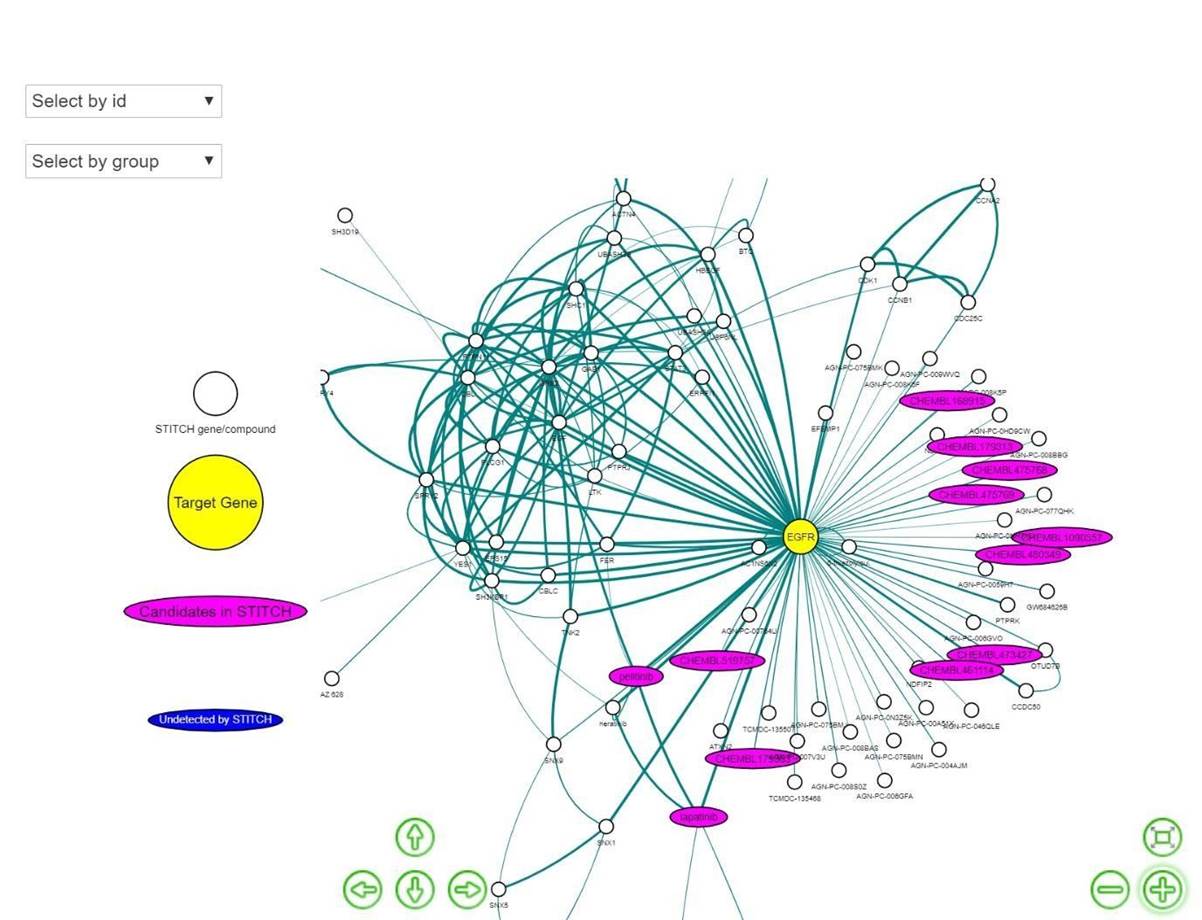
Figure 12. STITCH network analysis for EGFR, with interactions between the target gene shown as a yellow node and candidate compounds, including the user-added compounds and their LINCS similar analogs shown as the magenta nodes. The edges represent experimental and text mining-based evidence of interactions retrieved from the STITCH database.

Sig2Lead ranks potential inhibitors of a target gene by employing transcriptional signature connectivity and chemical similarity analysis

For a set of candidate molecules defined in a user provided file, candidate drugs are ranked by similarity to all LINCS analogs. LINCS

This tab permits clustering of concordant LINCS analogs and candidate compounds to determine classes of putative inhibitors

This tab utilizes known relationships of gene targets and small molecules to identify networks of LINCS analogs, candidate compounds, and gene targets.

Clusters or putative structural classes of top-ranking candidate molecules and their 'concordant' LINCS analogs are mapped into STiTCH drug-target network of known drug-target relationships.

Sig2Lead Overview